LSH applied to Transformer: The Reformer
Locality Sensitive Hashing (LSH) applied to the attention layer of a transformer reduces the inference time to almost linear
One of the main algorithmic tools I studied in my PhD was Locality Sensitive Hashing (LSH), so I was really surprised that only recently I got to know about its application to the Transformer architecture. This blog talks about Reformer: The Efficient Transformer, which introduced LSH in the attention block of the Transformer architecture to reduce the expensive quadratic inference time to almost linear in the context length. This paper, which comes from Google Research, received a lot of attention when it came out in 2020, but currently it is not implemented in state-of-the-art models, as the field preferred to focus on GPU-aware algorithms, like FlashAttention, instead of removing the quadratic inference time bottleneck. Thus, this blog is mainly for intellectual curiosity, driven by my research interest in LSH and state of the art deep learning architectures.
I will start with a brief introduction of LSH and attention mechanism, then I will expose how the two concepts can work together.
Locality Sensitive Hashing (LSH)
It is a technique based on hashing, which is a mathematical process to transform any input into a fixed-length code called hash. This is locality sensitive as the mathematical process is designed so that close inputs are mapped to the same hash, at least with some probability. This is essentially equivalent to organizing similar inputs into the same bucket. No wonder this tool was invented by researchers working on nearest neighbor problems. Here is the full definition:
Definition (Locality-Sensitive Hash Family). Let \((\mathcal{X}, d)\) be a metric space, and fix two distances \(r_1 < r_2\) and two probabilities \(p_1 > p_2\). A family of functions \(\mathcal{H} = \{h : \mathcal{X} \to U\}\) is called \((r_1, r_2, p_1, p_2)\)-sensitive if, for every pair of points \(x, y \in \mathcal{X}\) and \(h\) drawn uniformly at random from \(\mathcal{H}\):
\[d(x,y) \le r_1 \implies \Pr[h(x) = h(y)] \ge p_1\\ d(x,y) \ge r_2 \implies \Pr[h(x) = h(y)] \le p_2\]
Intuitively, we are looking for a family of functions such that, by randomly sampling a hash function from this family, close points share the same hash (same bucket) with probability at least \(p_1\) while far points do with probability at most \(p_2\). We are bounding the probability of the best and worst case scenarios. Notice that the hash functions themselves are deterministic; the probability comes from sampling randomly over this family of deterministic functions. This is worth mentioning, as it is often a source of confusion.
Constructing such families is not easy, and it depends on the metric space under consideration. On the unit sphere, the construction that both achieves the optimal exponent and is cheap enough to run is built from random rotations.
Cross-Polytope LSH Andoni, Indyk, Laarhoven, Razenshteyn & Schmidt, 2015 Let \(A\in\mathbb{R}^{d\times d}\) be a random matrix with i.i.d. entries \(A_{ij}\sim\mathcal{N}(0,1)\) (a random rotation). For \(x\in\mathbb{S}^{d-1}\), let \(y = Ax/\|Ax\|\), and define
\[h_A(x) = \argmax_{v \,\in\, \{\pm e_1,\dots,\pm e_d\}} y^\top v,\]i.e. the hash of \(x\) is the vertex of the cross-polytope \(\{\pm e_1,\dots,\pm e_d\}\) (the unit ball of the \(\ell_1\)-norm) closest to \(y\). The family \(\mathcal{H}=\{h_A : A\in\mathbb{R}^{d\times d}\}\) is locality-sensitive for cosine distance on \(\mathbb{S}^{d-1}\): for \(p,q\) at distance \(\tau = \|p-q\|\),
\[\ln\frac{1}{\Pr_{h\sim\mathcal{H}}[h(p)=h(q)]} = \frac{\tau^2}{4-\tau^2}\cdot\ln d \;\pm\; O_\tau(\ln\ln d).\]
The distance above is actually Euclidean, which is equivalent to cosine distance on the hypersphere, since \(\tau^2 = \|p\|^2+\|q\|^2-2p^\top q = 2(1-q^\top p)\). As you may have noticed, the smaller \(\tau\) is, the larger the collision probability is. Figure 1 makes this intuitive.
The \(2d\) vertices cut the sphere into \(2d\) identical wedges, and the \(\argmax\) just names the wedge you landed in. Rotating \(x\) by a random \(A\) is the same as leaving \(x\) alone and dropping the wedge boundaries onto the sphere at a random angle. Two points get different hashes only when a boundary falls between them, and the closer they are, the smaller the arc where one could. That is the whole mechanism, and it is represented really well in Reformer’s Figure 1.
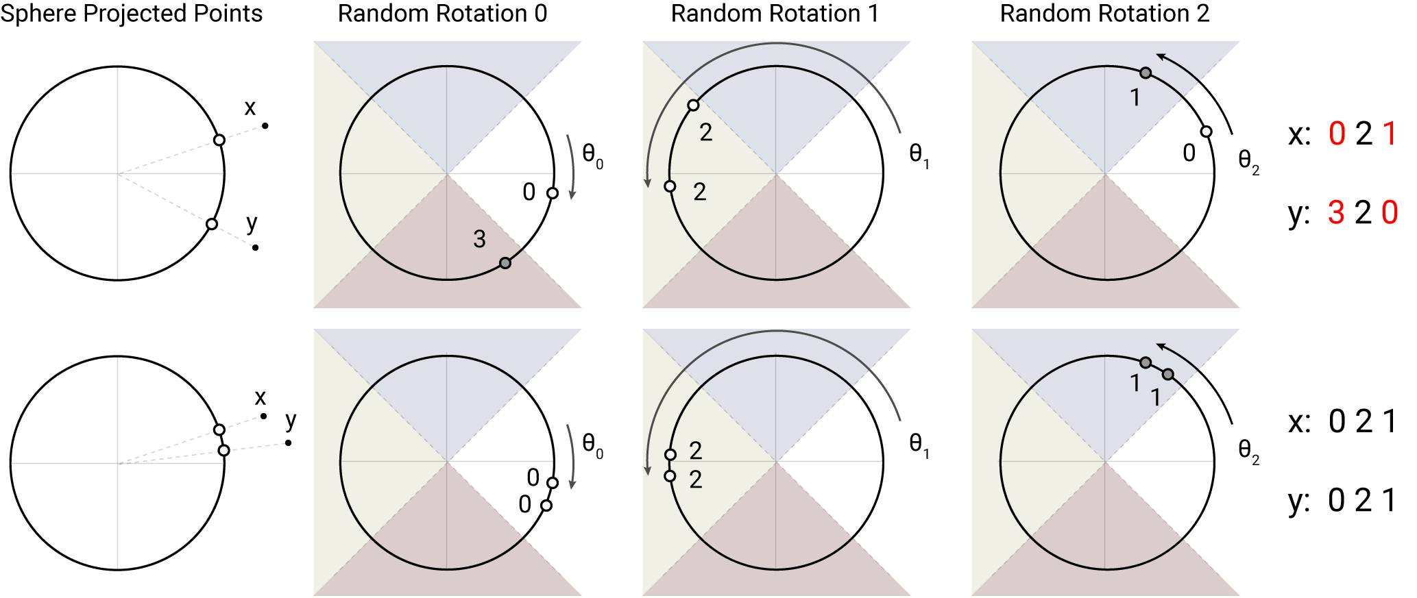
Figure 1 of Kitaev, Kaiser & Levskaya (2020), I believe it is a really instructive representation of cross-polytope LSH.
On the first row, the points \(x\) and \(y\) are far apart, and three rotations give them the codes 0 2 1 and 3 2 0. Look at the middle rotation: both landed in wedge 2, even though the points are nowhere near each other. In the bottom row the points are close and all three rotations agree. This example also highlights the need for concatenation in LSH, a technique to manipulate the probabilities \(p_1\) and \(p_2\).
Concatenation
Concatenating \(k\) independent hashes multiplies the collision probabilities: close points survive with \(p_1^k\), far points with \(p_2^k\). Since \(p_2 < p_1\) the far points decay faster and the buckets get purer, at the cost of losing close pairs at rate \(1-p_1^k\). The standard fix is to run \(r\) independent copies and take the union, which pushes the probability of finding a close point to \(1 - (1-p_1^k)^r\). Keep \(r\) in mind, it comes back later under a different name.
One practical note: multiplying by a dense Gaussian \(A\) costs \(O(d^2)\), so Andoni et al. replace it with a pseudo-random rotation using the Fast Hadamard Transform, which takes \(O(d\log d)\).
Self-attention
The self-attention module has three matrices, \(Q, K, V \in \mathbb{R}^{L \times d_k}\) (here, for simplicity, all sharing the same column dimension), where \(L\) is the context length and \(d_k\) is the dimension of the latent space.
\[\mathrm{Attention}(Q,K,V) = \mathrm{softmax}\!\left(\frac{QK^\top}{\sqrt{d_k}}\right)V.\]The bottleneck is \(QK^\top \in \mathbb{R}^{L\times L}\), which requires \(O(d_kL^2)\) operations to compute.
Now unwrap the same thing one query at a time:
\[o_i = \sum_{j \in P_i} \exp\!\big(q_i\cdot k_j - z(i, P_i)\big)\, v_j,\]where \(P_i\) is the set of positions query \(i\) attends to and \(z\) is the log-partition function (the normalization factor of the softmax). Full attention takes \(P_i\) to be everything. But the softmax is dominated by its largest terms, and those are the keys with the biggest inner product against \(q_i\); the rest contribute an exponentially small weight and get normalised away. At \(L = 64\text{K}\) the Reformer authors argue the 32 or 64 nearest keys may suffice.
So attention is a nearest neighbour problem! For each of \(L\) queries, find its closest set of keys among \(L\) candidates. LSH is built for this.
Putting the two together
Reformer sets \(P_i = \{j : h(q_i) = h(k_j)\}\), so a query attends only inside its own bucket. The hash is cross-polytope, written in the paper as
\[h(x) = \argmax\big([xR;\, -xR]\big),\]with \(R\) a random \([d_k, b/2]\) matrix and \([u;v]\) denoting concatenation. This is the same \(\argmax\) over signed axes as before, restricted to \(b/2\) of them rather than all \(d_k\), which is the “partial” cross-polytope. Its analysis is dimension-free, so the guarantee survives.
Shared-QK architecture
Queries and keys are hashed independently, and this leads to bucket imbalance.
- A bucket may contain a different number of keys and queries, so buckets do not pack into a fixed-length tensor, making batching across buckets difficult.
- Even worse, the number of queries in a bucket is unrelated to the number of keys in it, opening the possibility of a bucket with no keys at all!
To alleviate this problem, the authors proposed a shared-QK architecture. By setting \(k_j = q_j / \|q_j\|\), we solve the second part of the problem (though it is not really clear to me why normalizing by \(\|q_j\|\), as using instead any positive factor would not change the hash, which is sensitive to cosine distance). The worst case is now a bucket that contains only the pair \(q_j\) and \(k_j\). This choice also guarantees that every bucket contains the same number of queries and keys.
The first part of the problem is more subtle to solve, and it is easier to understand by looking at Figure 2. The queries are sorted by bucket number and, within each bucket, by sequence position to ensure causality. This lets us create chunks of \(m\) consecutive queries that attend to each other (this changes the sets \(P_i\) from what has been defined above). In practice, \(m = 2L/n_{\text{buckets}}\), which is twice the expected bucket size; the authors assume the probability of a bucket growing to twice its expected size is negligible.
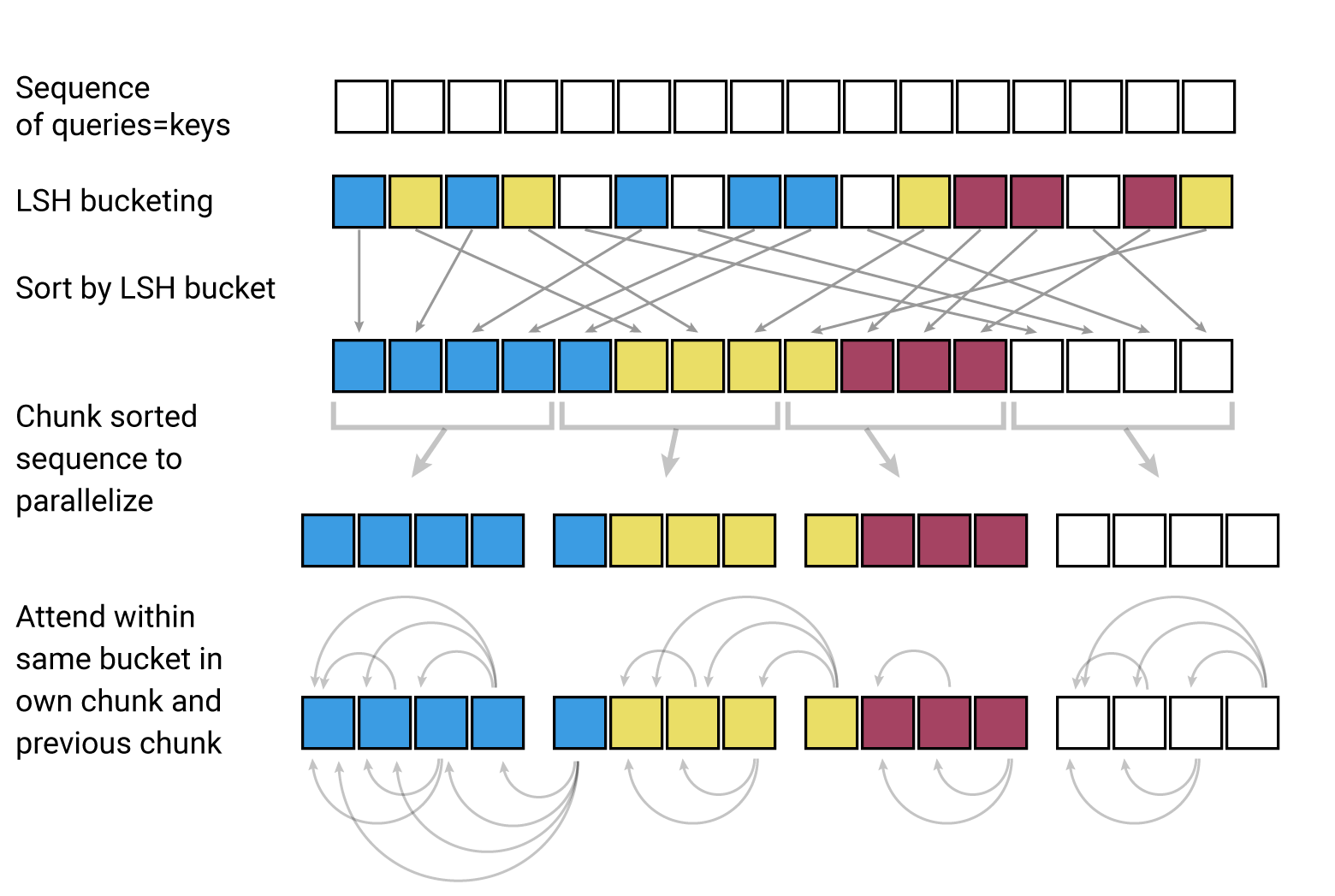
Left half of Figure 2 of Kitaev, Kaiser & Levskaya (2020): sort by bucket, then chunk into fixed-size blocks for batching.
With \(Q = K\), the dot product of a token with itself beats everything, so position \(i = j\) has to be masked out, except for a token with no other valid target (the worst case scenario).
The algorithm
The whole thing becomes four steps:
- Hash every position: multiply by \(R\). \(L\) hashes at \(O(d_k\, b)\) each.
- Sort positions by the pair (bucket id, sequence id) at \(O(L \log L)\).
- Chunk. Cut the sorted sequence into blocks of \(m\) consecutive positions. Each block attends to itself and to the one before it. Reformer sets \(m = 2L/n_{\text{buckets}}\).
- Repeat with \(n_{\text{rounds}}\) independent hash functions, taking the union \(P_i = \bigcup_r P_i^{(r)}\).
Step 4 is the \(r\) from earlier under a new name.
Adding it up:
| Step | Cost |
|---|---|
| Hash | \(O(L\, d_k\, b)\) |
| Sort by bucket | \(O(L\log L)\) |
| Chunked attention | \(O(d_k L\, m)\), with \(m\) constant by construction |
The chunk size is where the quadratic term goes to die. Reformer picks \(n_{\text{buckets}} = L/32\) so \(m=64\). The sorting step introduces the \(O(L\log L)\).
Where I would take this next
Everything above rests on \(Q = K\), and that constraint comes from using a hash. A hash is one function applied to both sides, so the only way to make a query and its key collide is to make them the same object.
A locality sensitive filter does not work that way. Here queries and keys are mapped using two different functions, the query filter and the update filter. In TensorTop-1, joint work with Martin Aumüller and Francesco Silvestri, we did something similar to cross-polytope LSH. Essentially, we sampled \(m\) Gaussian vectors \(a_1,\dots,a_m\) and treat the two sides asymmetrically:
- a data point (which might be a key) \(k\) is stored at the single filter it aligns with best, \(\argmax_i \langle a_i, k\rangle\);
- a query \(q\) opens every filter above a threshold, \(\{i : \langle a_i, q\rangle \ge \eta\}\), with
Where \(\alpha\) is the cosine between close points, a hyperparameter to be set.
Nothing there asks the query and the data point (key) to be the same vector, or even to pass through the same projection. Keys are stored, queries probe. This is exactly the asymmetric query/key treatment that Reformer had to give up for shared-QK.
The precondition to have a drop-in solution is that both sides live on the unit sphere. That used to be awkward to ask of a Transformer, but recently Nvidia developed nGPT which normalises every query and key to the hypersphere as part of the architecture. On such a model a filter-based attention would be a drop-in, with \(\eta\) as an inference-time knob playing the role \(n_{\text{rounds}}\) plays in Reformer.
This is just my intuition; there are many questions that need to be addressed, like how to properly batch this approach and how to deal with update filters that are empty. These are the same questions that led to shared-QK. I wonder whether locality sensitive filters end up being the better fit here. A drop-in solution for nGPT-like transformers would be quite something.