I finally implemented my own algorithm
TensorCloseTop-1 existed only as a proof. Now it runs. Here is what the theory got right and what it quietly hid.
There is a particular kind of guilt that comes with proving a theorem about a data structure you have never built. You know the guarantees hold. And still, somewhere in the back of your head, a voice asks: but does it actually run well?
The algorithm in question is TensorCloseTop-1, Algorithm 5 of Differentially Private High-Dimensional Approximate Range Counting, Revisited, joint work with Martin Aumüller and Francesco Silvestri, presented at FORC 2025. I finally sat down and implemented it, in Rust (this was a funny choice, but I said to myself, let’s try), with Claude as a pair programmer. This is what came out.
The problem - NNS and NNC and Approximate versions
You have \(n\) points on the unit sphere in \(d\) dimensions. Someone hands you a query \(q\) and you want to know: how many of my points are close to it? (NNC) or find me a point close to it (NNS). Close means inner product at least \(α\). In high dimension, answering this exactly means looking at everything, as the curse of dimensionality makes all the points likely to be orthogonal making them all equal to the search. So we relax the question in the standard way: if a point at similarity \(≥ α\) exists, we are allowed to return one at similarity \(≥ β\), for some \(β < α\). And then we ask for something harder: publish the counts in a way that is differentially private, so that no individual point can be inferred from the answers.
ANNS and ANNC refered respectivetly as approximate nearest neighbor search and approximate nearest neighbor count.
The (α, β)-ANNS-C problems, pictured
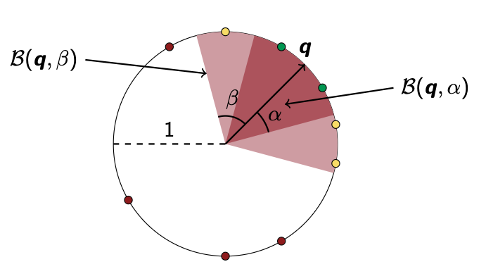
That is the unit circle standing in for the unit sphere \(S^{d-1}\): everything lives on the boundary, at radius 1 from the centre. Inner product similarity between two unit vectors is the cosine of the angle between them, so a similarity threshold is literally an angular wedge around \(q\) — the smaller the angle, the higher the similarity. Since \(β < α\), the wedge \(B(q, β)\) (light, wider) contains the wedge \(B(q, α)\) (dark, narrower) entirely. The green points sit inside \(B(q, α)\) (the close points), the yellow points are in \(B(q, β)\) but miss \(B(q, α)\) (the approximate close points), and the red points miss both (the far points).
The definition of \((α, β)\)-ANNS is the following: if at least one green point exists, return a green-or-yellow point — anything landing anywhere in the wide wedge counts as success. It never asks the algorithm to prefer green over yellow, or to identify which point is which. That slack, visible as the gap between the two wedges in the picture, is the entire relaxation the algorithm is built on: trade “find the closest point” for “find a point close enough,” and sub-linear query time in high dimension becomes possible.
Note: The condition if at least one green point exists is only necessary for providing theoretical bounds for the query time. In practice, this condition is not necessary and the algorithm returns any approximate close points.
The definition of \((α, β)\)-ANNC is similar but it does not require the existence of the green points: count any green point, may or maynot count any yellow point, but definetly do not count the red points. That is, any number greather than the number of green points, and smaller than the number of green and yellow points, satisfies the query. This query can be effectivetly answered privatley using differential privacy!
The idea
The tool is locality-sensitive filters. Draw a bunch of random Gaussian vectors and call them filters. A point gets parked at a filter when the two align well — their inner product lands high. Points close to each other tend to align with the same filters, so at query time you only need to open the filters that align with the query, and look at the handful of points parked there.
The catch is that the theory wants \(m = n^{\Omega(1-\alpha^2)}\) filters, which is far more than \(n\). You cannot store them. The trick that makes it practical is tensorization: instead of \(m\) filters, keep \(t\) independent groups of \(m_{sub}\) filters each, and give every point an address made of the \(t\) filter indices that caught it — one per group. That simulates \(m_{sub}^t\) buckets using the Cartesian product while physically storing only \(t · m_{sub}\) filters. At \(n = 10^6\) my implementation stores 5 223 filters to simulate 5.3 billion buckets. That is the whole magic trick.
The CloseTop-1 part is the paper’s own contribution: rather than parking a point at the filter it aligns with best (which forces you to reason about the distribution of a maximum), park it at the first filter whose inner product falls inside a narrow band. Bounding the alignment from both sides makes the analysis go through without any assumption about limiting extreme-value distributions.
Privacy then comes almost for free as we do not duplicate data in the data structure, so we can bound the sensitivity. Replace each bucket’s list of points by its size. Every point sits in exactly one bucket, so adding or removing one point moves exactly one counter by exactly one: the sensitivity is 1. Add truncated Laplace noise (obtaining approximate differential privacy) to each counter, publish, and answer queries by summing the noisy counters you land on.
Does it work?
Yes! But with some additional tricks.
Search. \(d = 128\), \(\alpha = 0.7\), \(\beta = 0.4\), 200 queries, every parameter taken from the paper’s formulas rather than tuned. Each query has one planted neighbour at similarity \(α\) hidden in uniform noise; in this dimension a random background point clears \(\beta = 0.4\) with probability \(≈ 3·10^{-6}\), so the yellow wedge of the picture above is, for all practical purposes, empty — the planted point is essentially the only thing anywhere near it. Success only requires landing in the wide wedge at all, not identifying the planted point specifically, but with nothing else there to land on, doing one means doing the other.
| \(n\) | build | success rate | buckets \(|I(q)|\) | non-empty visited | query |
|---|---|---|---|---|---|
| 10 000 | 0.04 s | 68.5% ± 3.3 | 17 455 | 54.6 | 0.094 ms |
| 100 000 | 0.94 s | 74.5% ± 3.1 | 318 554 | 278.1 | 0.910 ms |
| 1 000 000 | 29.2 s | 82.0% ± 2.7 | 5 552 064 | 1 326.4 | 7.300 ms |
The success rate climbing towards 1 as \(n\) grows accordingly to the \(1 - o(1)\) of the analysis.
Against brute force. I added an exact baseline — scan the points, return the
first one above \(\beta\) — because a sub-linear algorithm that loses to a for loop is a
paper, not a data structure.
| \(n\) | ANN | linear scan | speedup |
|---|---|---|---|
| 200 | 0.008 ms | 0.008 ms | 1.0× |
| 10 000 | 0.094 ms | 0.467 ms | 5.0× |
| 100 000 | 0.910 ms | 8.608 ms | 9.5× |
| 1 000 000 | 7.300 ms | 70.510 ms | 9.7× |
The crossover sits at about \(n = 200\). Above it the structure wins by 5–10×, and it wins for the reason the theory says it should: at \(n = 10^6\) a query covers 5.5 million buckets on paper, but only 1 326 of them contain anything, and only those get opened. The Cartesian product is a bookkeeping device, not a workload.
Memory. The overhead is real, and smaller than I expected: at \(n = 10^6\), 999 MiB of raw points plus 77 MiB of structure — 5 MiB of filters and 72 MiB of bucket index — for 7.8% over what storing the points alone costs. The \(O(dn)\) space bound is not just asymptotically true, it is true with a small constant.
Privacy. Now the counting structure, with 2 000 planted neighbours per query (true answer: 2 000), \(\delta = 10^{-6}\):
| \(ε\) | noise bound \(A\) | mean abs. error |
|---|---|---|
| 0.1 | 108.70 | 1 398.7 |
| 0.5 | 25.38 | 915.4 |
| 1.0 | 13.66 | 702.9 |
| 4.0 | 4.28 | 431.9 |
| 8.0 | 2.64 | 355.9 |
| — | non-private | 362.8 |
The last row is the one to read first. The non-private version of the same structure already has an error of 362.8, because the filters sweep in far points along with the near ones — that is the price of the \((\alpha, \beta)\) relaxation, not of privacy. By \(\varepsilon = 8\) the private answer has essentially reached that floor. Privacy is not what is costing you accuracy here; the approximation is.
What the theory did not tell me
Three things, all of which only appear once you run the thing.
The asymptotics hide a constant that bites. Lemma 23 says a point fails to collide with any filter with probability \(m^{-Ω(1)}\). Reassuring. In practice, at \(n = 10^5\) and \(m_{sub}= 502\), a single filter accepts a point with probability 0.0028, so a quarter of all points are dropped by each of the three groups — only 42.6% survive all three, and the success rate collapses to 34%. The fix (keep the stray points at their best-aligned filter, the Top-1 rule) restores 100% storage and 74.5% success, costs nothing in privacy, and is invisible asymptotically. \(m^{-Ω(1)}\) is doing a lot of quiet work in that lemma.
Worth to mention that this fix, the Top-1 rule, is exactly the asympotitc behaviour of CloseTop-1. It is interesting to see how things change in practice; CloseTop-1 is the mathematically correct but performs bad in practice, at least for a reasonable \(n\), while Top-1 is mathematically incorrect but performs good in practice.
The suppression threshold, not the noise, dominates at small \(\varepsilon\). To publish a sparse histogram you must drop small counters, or the mere presence of a key leaks membership. That means discarding anything below \(1 + A\). At \(\varepsilon = 0.1\) that threshold is 110, so only 2.9 of the 574 non-empty buckets a query touches survive, and the estimate collapses towards zero. The added noise is almost beside the point.
The \(|I(q)|\) term is a trap for the implementer. My first version enumerated the Cartesian product and did a hash lookup per key — faithful to the pseudocode, and hopeless: 318 554 lookups to visit 278 non-empty buckets. Sorting the bucket keys and walking them as a prefix tree gives identical answers 13.7× faster. The pseudocode is right; reading it literally is wrong.
Here I need to thank Claude for finding out this smarter and really faster implementation.
A note on the paper
I found a mathematical error in the paper that fortunately does not affect the asymptotic analysis. In Proposition 21 the right bound includes a factor \(1/2\pi\) on both left and right hand size. This changes Proposition 22 and Lemma 24 by just constant factor.
The code is on GitHub, with a README documenting every parameter,
the privacy argument, and how to reproduce all the numbers above. 45 unit tests,
cargo test.